Critical Dependence Stress for Portfolio Diversification
Abstract
We ask how much dependence uncertainty a diversification benefit can withstand when every marginal loss law is fixed. Our measure is the smallest weighted -Wasserstein perturbation that reverses the Expected Shortfall ranking of two nearby allocations evaluated under a common stressed law. For a positive continuous density on a compact box, exchangeability of the two traded positions eliminates the first-order gain, so the stress radius to study is for trade size . At this scale we obtain a -limit for the rescaled transport energies and prove convergence of the paired risk differences, with the two ES thresholds optimized separately. Coordinatewise quantile restoration incurs a marginal-flux cost, although its leading effects on the two ES values cancel in their difference. The limiting risk profile is continuous and strictly increasing, and its unique zero is the common leading coefficient of the budgets for a tie and for a strict reversal. We introduce the marginal-restoration premium, the excess of that coefficient over the local-efficiency lower bound, and prove that it vanishes exactly when background displacement is cheapest per unit change in portfolio loss. Otherwise it is strictly positive, even when the profile is exactly linear on an initial interval. For independent uniform losses on with , , and , the premium is at least of the local-efficiency bound. At equal effective costs, we characterize the right derivative of the critical coefficient with respect to the background penalty by continuous maximum-flow/minimum-cut duality.
I. Introduction
A risk desk may have agreed marginal models for its individual positions without an equally well-determined model for their joint losses with the background book [31]. That leaves open how much of a portfolio's diversification benefit survives uncertainty about dependence. We study the question by keeping the marginal models, letting the coupling change, and looking for the smallest dependence perturbation that reverses the Expected Shortfall (ES) advantage of a proposed reallocation when both allocations face the same stressed law. We develop a variational framework for this critical stress. It yields a critical-scale -limit, a common critical coefficient for a tie and a strict reversal, the marginal-restoration premium with its zero-premium classification, a flow–cut characterization, at equal effective costs, of the premium's sensitivity to background cost, and a uniform benchmark in which the asymptotic reversal budget is at least above the initial-slope prediction.
Let be the unit losses of two positions of equal initial cost. A transfer from holdings to , with an unchanged background loss , changes the portfolio loss from to , where
At upper-tail probability , we compare them through , optimizing the two ES thresholds separately under [32], so that favors the transfer under that law. The background term cancels from the payoff difference , yet we cannot drop it, because its dependence with the traded positions determines which states enter each portfolio's upper tail. A trade assessed in isolation can therefore rank differently once embedded in the whole book [8].
Writing for the Fréchet class of joint laws with these marginals, we measure distance from the reference law by weighted with ground cost , where each sets the budget penalty per unit coordinate loss displacement as losses are re-paired across joint states. At budget , the stress problem is
Under an exchangeable reference law the traded positions have equal marginal ES contributions, so the nominal gain is of second order: , with . When , for example, the local exchange in Proposition 2.2 attains an initial stress derivative of order one, which suggests the reversal budget . The derivative at zero budget does not determine whether this efficiency persists until the nominal gain is exhausted. The predicted reversal already sits at scale , so the tangent at zero is not enough, and we need the risk profile over a nonvanishing interval of the rescaled budget .
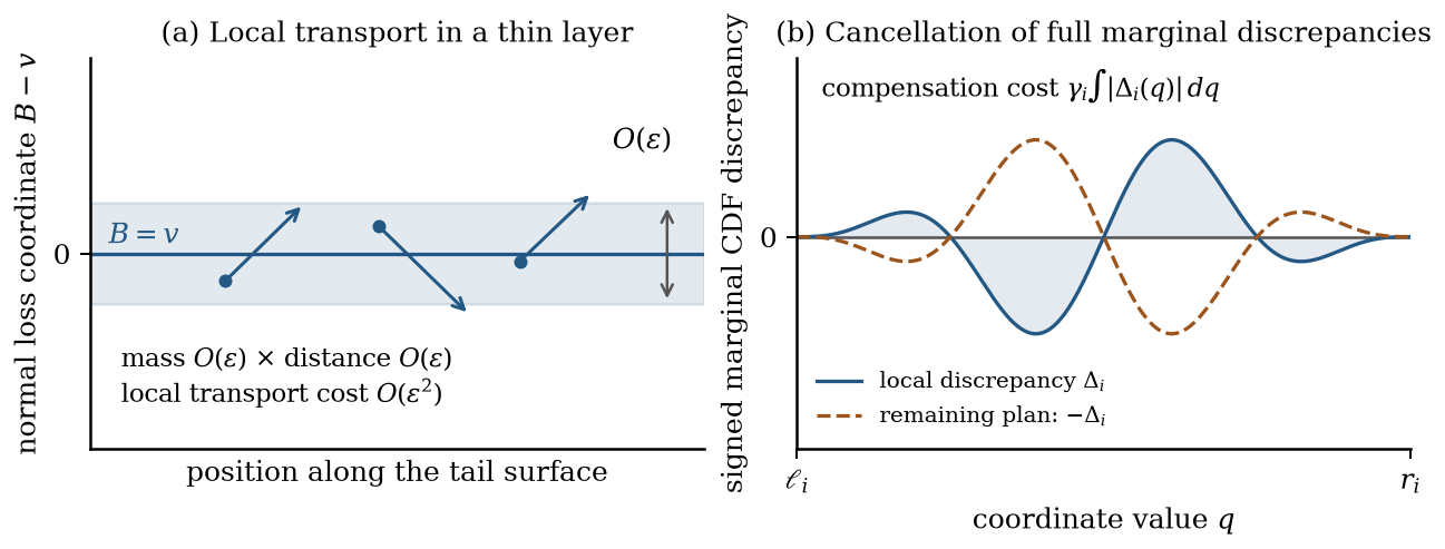
Three effects contribute at the critical scale. Moving the mass in an -layer around the reference tail boundary by distances of order changes both transport cost and tail expectation by , which matches the nominal gain. That local movement need not preserve the marginals, and restoring them has its own price. For a fixed regular local plan the marginal CDF discrepancies are , and by Vallender's formula [39] their norms give the one-dimensional restoration costs, even when compensation occurs far from the tail boundary. An shift of either ES threshold also contributes at order through the curvature of its objective. Since all three enter at the same order, we have to optimize the local displacement, marginal restoration, and both thresholds together.
Our main contributions are the following.
The critical-scale limit. When the reference law has a positive continuous density on a compact box and is exchangeable in its first two coordinates, Theorem 3.1 proves that the rescaled stress profile converges to a finite, continuous limit
with convergence locally uniform in . The proof rests on a -limit [11] of the transport energies that charges both for the local displacement and for restoring its marginal projections. In the recovery argument, coordinatewise quantile maps attain the restoration cost for each fixed regular local plan. This correction moves losses throughout the box, but its leading effects on the two ES values cancel outside the threshold layer, and approximation then extends the paired-risk convergence to kernels with finite displacement moment.
A common critical coefficient. Let and be the infima of budgets permitting a tie and a strict reversal. Theorem 3.3 proves that is strictly increasing with a unique zero , and that this zero is the common leading coefficient of both budgets, which gives the quadratic law for the critical stress:
The marginal-restoration premium. The effective unit costs are , and , with . If the first traded coordinate is cheapest, Proposition 3.2 constructs a positive interval on which . To reach zero at this rate, however, efficient displacement would have to stay possible throughout the required interval. We introduce the marginal-restoration premium, the nonnegative gap between the critical coefficient and the universal efficiency bound (normalized by when reported as a percentage), and Theorem 4.2 classifies exactly when it vanishes:
When background displacement is cheapest, exchangeability lets opposite shifts balance on every fixed-background slice. When only traded directions are cheapest, a corner region needs a displacement moment of order , while its coordinate projections admit only of compensating moment near the diagonal (Figure 2), so the premium is strictly positive. Under the attained-slope condition of Proposition 2.2, with , this mismatch gives , and (4.10) bounds this limit explicitly.
The uniform benchmark. Take independent uniform losses on , with , , and . Then and , so Proposition 2.2 gives . Corollary 5.2 proves that the profile is exactly for , yet its zero satisfies . So even in this uniform model, and despite an attainable initial slope, the marginal-restoration premium is at least : the lower bound we prove on reversal is above the local-efficiency prediction .
Flow–cut sensitivity at equal effective costs. Along the cost family , for , the baseline stays constant, so and the marginal-restoration premium have the same right derivative at . Here is the least background share among efficient stresses. Theorem 4.3 characterizes it by continuous maximum-flow/minimum-cut duality and writes it as a normalized supremum of projected cut deficits, and Section 5 shows how this share and the budget sensitivity can move in opposite directions as the reference dependence changes.
Our question lies between extremal risk aggregation and local distributional sensitivity. On the aggregation side, subadditivity bounds aggregate risk [1, 25], and rearrangements within a Fréchet class describe how diversification depends on the coupling [33, 15, 5, 16, 41]. Partial information leads to convex-order and mixability constraints [22] but can still permit comonotonic upper tails [12], and fixed-marginal MES bounds quantify uncertainty in individual tail contributions [9]. In allocation comparisons, the symmetry imposed on the candidate laws is decisive. Chen et al. [10] and Liu and Liu [23] use exchangeability and majorization to identify diversification protection, and Liu and Liu also analyze when complete dependence ambiguity favors concentration and how Wasserstein uncertainty modifies that conclusion. We impose exchangeability at the reference law alone: stressed couplings need not remain exchangeable, and the stationarity that symmetry gives at the reference does not by itself protect the reallocation once stress breaks the symmetry. We use this setting to measure the distance to a specified decision reversal, in the spirit of reverse sensitivity analysis [28, 29].
Transport duality is a natural way to preserve the marginal information [40, 34]. In Wasserstein robust optimization [7, 19], adding marginal constraints confines the perturbation to dependence changes [18, 13]; such constraints encode calibrated risk-neutral laws in multiasset robust pricing [14], and Wasserstein and copula restrictions also arise in benchmark portfolio optimization [30]. Here the constraint acts on a common stressed loss law for two allocations. After rescaling, its full coordinate projections remain as a transport penalty, and at equal effective costs we show that the efficient allocation of displacement reduces to a capacity-constrained flow problem [20].
Local Wasserstein expansions relate the sensitivity of optimized decisions and AVaR criteria to changes in the reference law [2], and adapted transport brings in the information available in multiperiod decisions [4]. When a first-order term vanishes, one turns to higher-order expansions: Fiechtner and Blanchet [17] derive a second-order regret expansion under a unique empirical-risk minimizer in this situation, and Sauldubois [35] develops higher-order Wasserstein and adapted-Wasserstein expansions, including martingale constraints. Dependence restrictions also affect local sensitivity, as in Lam [21], while Namkoong [26] evaluates the first-order response over restricted transport directions. In our problem the trade size and stress radius vanish together, so locating a decision reversal at scale takes the full rescaled profile, which Theorem 3.1 gives with global marginal compensation and both optimized ES thresholds retained over the budget interval needed to reach zero.
Section 2 derives the nominal gain and the initial stress slope, and Section 3 takes the variational limit at scale and identifies the unique zero of the limiting profile. Section 4 characterizes zero premium and represents the boundary derivative by continuous projected flow–cut duality. Section 5 works through analytical examples and what they imply for reverse stress testing. The analytic proofs are in Appendix A, and the potential estimates and section calculations for the examples are in Appendix B.
Notation and conventions We write for a pushforward and measure displacements by . The constant in may depend on the fixed kernel and model, but not on . Scalar section integrands are extended by zero outside their domains, and projection identities are equalities of finite signed Borel measures. We use ; allocation ratios are assigned the value zero where both numerator and denominator vanish.
II. Model formulation and the local benchmark
We first formulate the comparison for arbitrary integrable marginal laws, which are enough for a worst stressed model to exist. The critical-scale analysis will use a positive continuous density and exchangeability of the two traded positions, both introduced in Section 2.2.
A. Fixed marginals and a common stress law
Let , let have finite first moments, and fix in the Fréchet class .
For exposure vectors , the losses before and after the proposed reallocation are and , with and . We use the upper-tail mass and the Expected Shortfall representation of Rockafellar and Uryasev [32],
We write for the threshold objective. For an integrable loss, its minimum is attained on the nonempty compact interval characterized by
Without a continuity assumption on the stressed loss law, support gaps can leave a nondegenerate interval of minimizing thresholds. We therefore keep the set-valued characterization (2.2), so that subsequent estimates apply to every minimizer, including for laws with atoms.
Under a common candidate law , we compare , minimizing each loss over its own threshold. Maximizing this paired difference tests whether a single dependence scenario can erase the nominal gain, whereas separate maximizations of the two ES values may select different joint laws. We measure changes in dependence with positive weights and ground cost
Within , transport changes how component losses are paired across joint states. With the weights and all marginal laws held fixed, we define the worst comparison at budget and the nominal gain by
Proposition 2.1 guarantees attainment in (2.3), allowing atoms, singular dependence, and unbounded marginal supports. A nondecreasing profile can vanish on a whole interval, so we distinguish the infimal budgets for a tie and a strict reversal,
which, by Theorem 3.3, have the same leading asymptotics in the exchangeable box model of Section 2.2.
Proposition 2.1 (Existence under integrable marginal laws). Let , let have finite first moments, and fix , positive weights , exposure vectors , and . Then and every are compact for , and the maximum in (2.3) is attained. For each fixed , the profile is nondecreasing and Lipschitz on .
Proof. The fixed-marginal class is tight and weakly closed. Moreover, along any weakly convergent sequence in , the first moments satisfy , so the Wasserstein convergence criterion [40] implies -compactness of and its closed subsets . For a linear loss , coupling the laws and minimizing the uniformly Lipschitz hinges over their thresholds gives
Applying this bound to and , we find that their ES difference is Lipschitz with constant . Compactness of then ensures attainment. To compare two budgets , take a maximizer at . The mixture , , satisfies and , by mixing an optimal plan with the corresponding identity plans. Comparing and yields . Q.E.D.
For a transfer between positions with the same marginal law, replacing by preserves every marginal and gives at cost ; reversing their roles yields
So the tie budget is finite, but this bound leaves its small-trade scale open. Under the exchangeable box assumptions introduced next, Section 3 shows that both critical budgets are of order .
B. The exchangeable box model
To isolate how dependence with the rest of a portfolio affects a small reallocation, we keep the two traded losses separate and collect all unchanged positions into their aggregate loss . The marginal law of counts as retained information, and we specify the transport metric directly on . This aggregate model fixes the information used in the stress test: the retained marginal and displacement cost are those of the aggregate loss, a different specification from fixing separately the marginals and transport costs of every underlying background position.
Standing assumptions (exchangeable box model) Let
We also write when treating coordinate projections together. The reference law has a continuous density on the closed box , normalized to integrate to one and satisfying . We take
with arbitrary and , so that and in the preceding notation. All model parameters remain fixed as . The first two unit positions are expressed at equal initial cost, allowing the trade to change their holdings from to without changing the initial outlay. The position represents the background book, whose holding remains unchanged during the trade.
The stressed law may be any coupling in ; exchangeability and absolute continuity are assumptions on the reference law only. Reference symmetry makes the equal allocation stationary under , and equality of the first two marginals gives under every candidate, so before implementation costs the ES comparison distinguishes tail risks between portfolios with the same expected loss.
We work on a compact box with a positive continuous density because that lets us study this dependence mechanism with uniform control of marginal restoration. Positivity on the closed box gives both the interior mass that local exchanges need and lower bounds on the marginal densities, hence Lipschitz bounds for their inverse CDFs, and these bounds enter the quantile recovery in Section 3.2 and Appendix A.5. Section 5.3 takes up the additional difficulties posed by unbounded marginals.
Loss units and effective stress costs A shift changes the portfolio loss by at cost . So , , and are the costs per unit change of along the three coordinate axes, and the ratio compares a background displacement with a first-position displacement having the same effect on portfolio loss.
Canonical box normalization Writing the original coordinates as , with and , gives a normalized model on with and . By cash invariance and positive homogeneity of ES, the original paired risk is times its normalized counterpart, while corresponding transport plans have equal cost; hence the critical budgets agree and is unchanged. A common rescaling of all transport weights rescales those budgets.
C. Nominal curvature and the exact initial slope
Under the reference model of Section 2.2, let be the upper-tail threshold of . The marginal expected shortfall (MES) of a unit position , namely , is the ES derivative with respect to its holding, and multiplying by that holding gives its Euler contribution [36, 38]. The first two holdings in both equal one, so the directional derivative along is their MES difference: with , it equals by exchangeability. To find the gain from a nonzero trade we then have to differentiate the moving tail boundary, which leads to a conditional variance on the tail section.
We record the classical section differentiation formula under our continuity assumptions in Lemma A.1.
The tail boundary can be parameterized by
Since and , the threshold satisfies . To locate a nondegenerate part of the section, follow the segment joining the lower and upper vertices of . The loss increases strictly along it and crosses at an interior point , so a neighborhood of lies in , and its points off the diagonal have .
By the coarea formula, integration in the normal coordinate gives the section measure . We denote the density of at and the nominal gain coefficient by
Here is the loss density at the threshold, and is its normalized conditional section law. Exchangeability makes the conditional mean of zero, giving , so the second-order diversification gain is governed by the conditional variance of the trade payoff on , weighted by the threshold density .
Proposition 2.2 (Nominal benchmark and exact initial efficiency). In the exchangeable box model of Section 2.2:
(i) Nominal gain and threshold curvature. The reference thresholds and nominal gain satisfy
The threshold of is unique for every , and for . With , the unoptimized objective satisfies, uniformly for and ,
(ii) Fixed-marginal Lipschitz bound and initial slope. For every ,
For fixed , if
then there exists such that
Proof. For part (i), the coefficients of are positive whenever , and its support is . Since every interior level meets , Lemma A.1 gives a positive continuous loss density and a unique threshold. The gradients of and are linearly independent, so is nonconstant on each such section. Its conditional variance is therefore strictly positive, and the same lemma implies strict convexity of on .
At , exchanging the first two coordinates preserves both the reference tail and its boundary measure and reverses , giving . In the notation of Lemma A.1, the remaining section moments at are and . Thus the threshold derivative vanishes and the optimized second derivative is , which yield (2.6) by Taylor expansion at zero. Strict convexity makes this stationary point the strict minimum, so for all . For the unoptimized objective , the Hessian at is . Expanding at the trade size and threshold displacement gives (2.7), uniformly on bounded -intervals.
The fixed-marginal Lipschitz bound. We next establish the uniform Lipschitz bound over . Given any minimizing for under and any minimizing for under , let
Both gaps are nonnegative, and direct subtraction gives
A direct bound on would use its largest absolute -slope, . Because and share their marginals, adding an integrable separable potential does not change the integral against . We can thus choose a representative of modulo marginal potentials with a smaller Lipschitz bound. Here the required adjustment is linear: since , we may add any scalar multiple of . The extreme -slopes, and , have midpoint , so adding minimizes their largest absolute value among constant shifts and simultaneously centers the -slopes. Away from the two tail planes, the four regime slopes are
With the extreme -slopes centered at zero, their largest absolute value drops to , while the corresponding bounds for and are and . Setting , which is absolutely continuous along coordinate lines, we obtain
Integrating against an optimal transport plan and then interchanging proves (2.8). The mixing argument in Proposition 2.1, now with this sharp constant, also gives
Attaining the initial slope. Under (2.9), we construct an attaining exchange near an interior intersection of the reference tail planes and . To locate such an intersection, fix and let be the nondegenerate range of on . Both losses increase along each nonconstant segment from the lower vertex . Any point with lies beyond an intersection of that segment with , so would imply . Since is nonconstant on , the second tail would also contain an open set below , contradicting the equal tail probabilities and . Rays toward the upper corner similarly exclude , which leaves . The relative-interior property of a linear map on a convex section gives an intersection .
To exchange the first-coordinate marginal intervals of two small source cubes in opposite disagreement regions along , we first choose reference points with the same coordinate and seek equal and opposite changes in the two losses. From the interior intersection , a displacement changes by and by . Equating their sum to zero determines . Thus the points
have opposite strict tail memberships for small : at , the losses differ from their thresholds by for and for , with both signs reversed at . Choosing bounds the loss change along either half-translation by the strict tail margin. With this margin fixed, we can take small enough that the cubes of half-width , centered at , have disjoint second-coordinate intervals and remain inside and their respective tail regions throughout translation by .
The uniform subdensities , where , have equal mass and sum at most . The translations therefore define the admissible perturbation
The translations exchange the first-coordinate marginal intervals, fix the other coordinates, and cross neither tail plane. Thus preserves all marginals and both reference tail probabilities, leaving and optimal. Integrating the affine hinges on the two cubes gives
The plan has cost , and the sharp bound (2.8) forces this to equal . Varying proves (2.10) with . Q.E.D.
If and , condition (2.9) holds for every , which suggests the extrapolated reversal budget . The construction gives for each fixed trade size, but the disagreement regions narrow with , so it leaves uncontrolled. Indeed, the unscaled bound makes both iterated limits in vanish even though , which is why Section 3 tracks the profile under the joint scaling .
Reference symmetry and stressed dependence Our stress class allows asymmetric dependence between the two traded positions. If every candidate law were exchangeable, the losses and would have the same distribution, and convexity of ES would give
Requiring exchangeability of every stressed law would thus protect this reallocation [10, 23]. We impose it only at the reference, which gives stationarity there while permitting dependence stresses that test the persistence of the gain. Identical marginal laws alone do not imply stationarity. For example, on with and , the perturbation , with , preserves uniform marginals but gives a nonzero tail expectation . Antisymmetry in preserves the law of , hence . Pairing leaves the strip , so
III. Variational limit and the critical profile
Under the traded-coordinate condition of Proposition 2.2, a local exchange attains the initial slope. To find out how far that efficiency persists toward reversal, we now hold fixed. The limiting objects introduced below connect the stress profile to its reversal coefficient:
The first passage comes from Theorem 3.1, which combines convergence of the transport energies with exact marginal recovery and convergence of the paired risk. Strict growth in Theorem 3.3 then identifies the common critical coefficient.
A. Local transport and marginal compensation
An -layer around contains reference mass, so displacements of order change both the transport cost and the paired hinge expectation at order . We resolve this layer through the normal coordinate and displacement , while keeping the cost of any transport outside bounded windows that is needed to restore the marginals.
Definition (Marginal flux and effective energy) On bounded -windows the rescaled source converges to . We disintegrate a limiting plan with this source into a probability kernel , specifying the rescaled displacement at surface point and normal coordinate ; stationary sources have kernel . Writing , we require a finite weighted displacement moment even though the source measure has infinite total mass:
Across a coordinate cut , upward movements remove mass from below the cut and downward movements add mass to it. The resulting signed flux has a Lebesgue density , as shown by the section formulas in Appendix A.3, and we define
In words, is the signed displacement moment projected onto the -th coordinate, and its negative is the leading marginal CDF discrepancy produced by a regular local plan. The full plan preserves each marginal, so transport outside a bounded normal and displacement window has to compensate the discrepancy within it, and the one-dimensional CDF formula for [39] turns that compensation into a cost lower bound. The energy adds this limiting restoration cost to (Figure 1). Projection contracts total variation, giving , with when all projected fluxes vanish and when each has a fixed sign -almost everywhere, so that .
B. The limiting risk and convergence theorem
Under the same local plan, each loss has its own minimizing threshold. At threshold , a displacement changes the leading centered and rescaled loss of from to . Denote the corresponding hinge increment by . We write for its integral.
Definition (Limiting paired risk) Moving the threshold away from contributes the curvature term from (2.7). Adding the local transport increment gives the two limiting threshold objectives, which must still be minimized separately:
The energy depends only on the absolute displacement moment and the signed coordinate projections, and it is convex under mixtures of kernels. The paired risk also depends on how the displacements are distributed relative to the normal coordinate : each of the two hinge objectives optimizes its own threshold, so their difference need not be concave in the common kernel.
We omit the superscript when the kernel is clear, and write , . Since , the quadratic term gives coercivity and confines every minimizer to . Together with convexity from Lemma A.4, these properties justify the threshold minimizations in . We then optimize the paired value over the energy budget, with attainment proved in Theorem 3.1:
We use vague convergence on , testing against compactly supported continuous functions on , so that compensation may occur outside bounded windows. We lift a plan from to a law in by
Here the factor compensates for the thickness of the source layer. The lifted coordinates determine for fixed , so the rescaled energy can retain the cost of the entire original plan:
Here we identify with a measure on through , using on and assigning zero measure to . Because includes the whole plan, including transport outside bounded normal windows, minimizing it over plans with target law gives . We formulate the following -convergence statement in this vague topology [11].
Theorem 3.1 (-convergence and the critical risk profile). Consider the exchangeable box model of Section 2.2.
(i) Transport plans and compactness. -converges to as in the vague topology on . Every sequence , , with bounded has a vaguely convergent subsequence. If has bounded energy and is the target law of , then .
(ii) Target laws and exact recovery. For every sequence and every feasible sequence satisfying , there are a subsequence and a kernel with finite such that
Conversely, every kernel with finite admits a recovery sequence of distributions preserving the original three full marginals, with
(iii) The stress profile. The maximum in (3.3) is attained. The function is finite, continuous, and nondecreasing, with and at some finite budget. For every finite ,
Proof strategy Theorem 3.1(i) gives -convergence of the transport energy and convergence of the paired risk along bounded-energy plans, and the exact marginal recovery in part (ii) makes the limiting kernel values asymptotically attainable in . Part (iii) gives uniform convergence of the optimized profiles on compact budget intervals, which, together with the strict crossing in Theorem 3.3, locates the reversal budget .
Step 1: Localization and the energy lower bound. Because the two ES thresholds are optimized independently, comparison of the objectives requires a common threshold window for stresses with bounded rescaled energy. In Appendix A.2, Lemma A.2 places every minimizing threshold in an window. On bounded windows the lifted plans are locally compact; outside them, marginal conservation requires compensation for the projected local flux. The compensation bound above then gives the energy lower bound for arbitrary admissible plans. Choosing optimal plans yields the corresponding Wasserstein bound for their target laws.
Step 2: Convergence of the paired risk. Bounded first moments make each hinge increment integrable, but need not give uniform integrability along convergent plans. The two objectives share the same large-displacement contribution, so we subtract from both. The relative increments are bounded on the common threshold window. Outside a normal window enlarged to account for the bounded reallocation , a nonzero relative increment requires a sufficiently large displacement, so the first moment controls the far-field contributions. The baseline integral is finite but need not converge. Since it translates both threshold objectives by the same amount independently of the threshold, it cancels exactly from their difference of minima.
Step 3: Exact marginal recovery. Let denote probability kernels with compactly supported continuous weights on finitely many fixed displacement vectors and the remaining mass at zero, as in (A.13). For a fixed kernel in this class, local translations yield a preliminary law with uniform marginal CDF expansion , where is the reference CDF. The quantile maps restore all three marginals at cost , with displacements.
To see why this correction does not alter the leading paired risk, compare its displacement scale with the threshold band. Outside a sufficiently wide band, the paired hinge has gradient above both thresholds and zero below both, so multiplying by the restoration displacement gives an contribution. Inside the band the gradient is bounded, but the -mass is only , giving the same order after integration. The restoration error is therefore , uniformly over all minimizing threshold pairs.
Approximation by in cost, paired risk, and the vague plan topology (Appendix A.4), followed by diagonal recovery, gives the general error. Compactness, contraction toward the identity, and the common budget-Lipschitz bound then give locally uniform convergence of the optimized profiles.
C. Initial linearity and the critical budget
At zero threshold shifts, the portfolios disagree on tail membership precisely on . The displacement moves a source in this wedge to the limiting -boundary and attains the maximal paired hinge increment per unit of normal movement. When , we can assign this movement along provided its downward and upward moments balance on each -fiber. On active sources in , for and for , with . Writing , the available fiber moments are
Exchangeability gives , but the two moments need not agree on each fiber. Matching their pointwise minimum cancels the projected flux and gives the budget
Proposition 3.2 (Capacity of the initial linear segment). In the exchangeable box model of Section 2.2, suppose . With as in (3.7) and as above,
Proof. For and , select the proportion
and define for . Because and the active sources satisfy , this is a finite-first-moment probability kernel. Its opposite first-coordinate fluxes equal and , while the other coordinates remain fixed, so for all and .
Under this displacement, an active source has target normal losses for and zero for . Because on , its strict -tail membership is unchanged and no mass is placed at the -threshold. For , however, the active sources from the two signs of arrive at the kink itself. The resulting atom accounts for the jump between the one-sided derivatives: with ,
By Lemma A.4, zero is globally optimal for both objectives. Evaluating the nonzero wedge integrals, for on and for on , we obtain and , which yield . Since by Lemma A.3, we may choose to attain the upper bound inherited from Proposition 2.2. Q.E.D.
Strict growth To identify a common leading budget for a tie and a strict reversal, we improve every bounded-first-moment kernel at arbitrarily small additional cost. If the paired risk were concave in the kernel, mixing with a kernel of larger paired risk would do this directly, but the two threshold objectives are minimized separately and their difference need not be concave along mixtures. We also cannot assume that a kernel leaves stationary mass available for an added displacement, since an everywhere nonzero shift proportional to already has finite first moment.
We instead replace a small fraction of the existing kernel on two exchanged normal bands beyond the common threshold window. Reflecting to crosses that window. Pairing the bands cancels their -increments, while opposite signs of produce a positive paired gain per unit replacement fraction, independent of the distance . After subtraction of the common baseline the old kernel contributes only an remainder, because it takes a large displacement to affect the threshold window from those bands. So we first choose to make this remainder smaller than the reflection gain, and then reduce the replacement fraction to meet the additional budget. Appendix A.6 verifies the mixing obstruction and carries out this comparison uniformly over the original and modified minimizing thresholds.
Theorem 3.3 (Strict improvement by local replacement and a common critical coefficient). Consider the exchangeable box model of Section 2.2. The limiting profile is strictly increasing and has a unique zero , which gives the common leading coefficient of both pre-limit critical budgets at scale . More precisely:
(i) Quantitative local improvement. For every there exists such that every kernel satisfying and every admit a feasible kernel with
These kernels can be chosen as a family satisfying
For every finite ,
(ii) Critical budgets. Together with the continuity, negative initial value, and positive value at a finite budget in Theorem 3.1(iii), strict growth of gives a unique zero . Over the finite-first-moment kernel class,
The corresponding pre-limit critical budgets satisfy
The first two minima are attained, whereas the infimum over strictly positive risk values is not.
Execution costs A positive execution cost proportional to exceeds the second-order nominal gain for small trades. To retain a critical-budget comparison, suppose instead that the deterministic cost paid to implement the new allocation satisfies and . With the stress class and metric fixed, cash invariance gives , whose rescaled profile converges locally uniformly to .
Applying the tie and strict-reversal definitions in (2.4) to the net profile, we obtain by strict growth and local uniform convergence , where is the unique solution of . As the rescaled execution cost increases to , this solution decreases continuously from to zero. For example, in the cheap-background case of Section 4.1, the explicit linear profile gives .
IV. Efficiency premiums and projected flow duality
We now ask when the critical coefficient reaches the local-efficiency lower bound and when a strict marginal-restoration premium remains. A locally efficient displacement need not preserve the marginal projections, so any unbalanced moment has to be compensated elsewhere. We measure this obstruction by testing each projected flux against a bounded measurable coordinate potential, using the dual representation of the restoration cost:
Here acts as a dual shadow price for the projected displacement moment at coordinate level . For the projections to vanish, opposite signed displacements have to balance at each coordinate level, and then the leading restoration penalty disappears. We first identify the pointwise displacement required for equality in the efficiency bound, and then test its projections near an off-diagonal corner to rule out equality when only traded coordinates are cheapest. At equal effective costs, continuous potentials lead to the flow–cut duality of Section 4.2, and allowing nonzero projected fluxes in the restoration-cost bound leads to the piecewise-constant potential estimates of Section 5.1.
A. Local efficiency and the zero-premium classification
With , , , and , Proposition 2.2 and Theorem 3.1 already give . The issue at zero risk difference is whether a kernel can satisfy the pointwise efficiency conditions while conserving every marginal projection, and we characterize those simultaneous equality conditions below.
Proposition 2.2 gives initial efficiency at each fixed trade size under (2.9), and when , Proposition 3.2 separately realizes the limiting slope by matching opposite first-coordinate moments on each fiber. When only traded coordinates are cheapest, that matching is enough for the initial linear segment but cannot cover the whole tail section. If the background coordinate is cheapest, exchanging and reversing instead balances the required displacement on every background slice, which sustains the efficiency bound up to zero risk.
Lemma 4.1 (Local-efficiency bound and critical-level optimality). In the exchangeable box model of Section 2.2, every kernel with satisfies , so . Set and . Then if and only if there is a measurable probability kernel satisfying
Such a kernel has and ; every kernel with and satisfies these conditions.
Proof. Set , , and choose any . To compare the risk gain with its transport cost, we evaluate the -objective at zero, bound the difference of hinge increments by , and use . Recording the loss in each comparison gives
The five terms (I)–(V) in (4.2) have distinct roles: (I) the marginal-restoration penalty; (II) the excess transport cost over the cheapest normal movement, including cancellation between coordinate displacements; (III) the curvature cost of shifting the -threshold; (IV) the unsaturated hinge gain; and (V) the gap from evaluating the -objective at zero instead of its minimum. For the fourth term, , an interval of length , so the difference of the two hinge increments cannot exceed . All five terms are consequently nonnegative, proving the efficiency bound. Since was an arbitrary minimizer, equality forces each defect to vanish for every optimal -threshold.
To reach zero risk at the local-efficiency budget, none of these defects can remain. Indeed, if and , the left side of (4.2) is nonpositive, so every nonnegative term must vanish and
In addition, and . The vanishing metric defect
allows only cheapest coordinates, with all nonzero components having the sign of . At , equality in the hinge bound requires , if , and , if . Thus , with the sign of wherever . Since
and every conditional kernel has mass one, . Saturation of this nonnegative bound forces
which, with the metric and flux equalities, proves necessity.
For the converse, the threshold calculation depends only on the normal displacement . We integrate over the disagreement wedge and use exchangeability to obtain
Because the transformed -loss retains its strict tail sign and places no atom at zero, we have . With , the mass placed at the -threshold kink gives
By convexity, these strict one-sided inequalities make zero the unique minimizer of . For , the stationary regions and each have section mass , and their unchanged normal coordinates cover the positive and negative half-lines, respectively. Hence on , and Lemma A.4 yields , so zero is also the unique minimizer of . Combining these minima with (4.7) gives . Under (4.1), we have and vanishing fluxes, so . Together with attainment of the critical cost in Theorem 3.3, this proves the equivalence. Q.E.D.
If , the profile is explicitly for .
If and , then
where is the projected imbalance of Section 3.3.
Proof of Theorem 4.2.
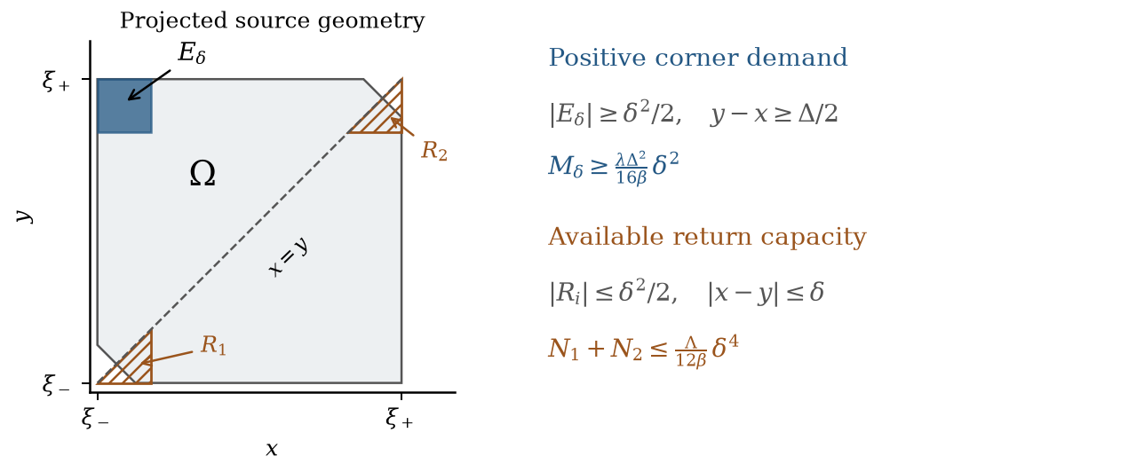
By Lemma 4.1, it suffices to allocate the prescribed displacement among cheapest coordinates while preserving every marginal projection. The background coordinate admits such a balance because exchanging the traded losses and reversing the normal coordinate leaves each background slice fixed and reverses the required displacement. For the traded coordinates, the corresponding balance must instead be found along each - or -fiber. Near an off-diagonal corner, the required moment is bounded below by a positive multiple of , whereas the opposite-side sources available at those coordinate levels have capacity only . We prove the background construction first and then use this discrepancy to exclude even randomized splitting among the traded directions.
Comparison kernels and the sufficient direction Assigning the prescribed displacement to one coordinate gives
with finite first moments and zero risk differences by the normal-displacement calculation (4.7)–(4.8) in Lemma 4.1. The first two kernels have respective fluxes and , all other fluxes being zero. To verify the background projection, we use the exchange , which preserves and reverses . Absolute integrability then allows us to test against every bounded measurable , obtaining
All three projections of vanish, yielding
The background kernel proves sufficiency, including ties, and the least of these costs gives , which yields the upper bound in (4.10) when and .
When , mix the background kernel with the identity using weight . Both kernels have zero projected flux and both threshold objectives attain their minima at zero, by (4.7)–(4.8) and , so cost and paired risk are affine along the mixture. Its cost is , and (4.7) gives
Thus the mixture attains the efficiency bound on the stated interval.
The obstruction for arbitrary randomized kernels For necessity, suppose and a kernel with attains cost . Lemma 4.1 then requires , , and both traded components to have the sign of . Since the kernel has finite first moment, its averaged displacement fields , , are integrable on the section and satisfy, by (4.1),
Projected conservation gives, for every pair of Borel sets ,
We test (4.15)–(4.16) near the upper-left off-diagonal corner of , where is small, is large, and the positive moment is bounded away from zero. Compensating this moment at the same coordinate levels requires negative moment from , where the small value of or large value of confines available sources to a small triangle near the diagonal (Figure 2).
The section base is the intersection of an open square with a diagonal strip, , whose boundaries and coordinate projection endpoints are
Both coordinate projections of equal , and the interior diagonal point from Section 2.3 satisfies , confirming . In addition, , so the corner lies in the closed strip, possibly on its boundary. The square diagonal through that corner runs parallel to the strip boundaries. On the corner square , , the strip condition reads . Because the two nonnegative slacks sum to , at least one is at least . Choosing therefore includes one of the triangles and . If we also choose , we obtain
Because is bounded below on and on this region, there is a constant , independent of , such that
Testing (4.16) on and requires , where
In , the conditions and force ; in , the sources similarly satisfy . Each triangle has area , and (4.15) bounds the corresponding displacement moment by . Applying the upper density bound gives
Here is independent of . For small , the bound contradicts . Attainment of the critical cost then implies when , and (4.13) gives (4.10). Q.E.D.
B. Boundary sensitivity and the flow–cut representation
At equal effective costs, every efficient kernel has total required displacement . At this critical level, the equality conditions and total-moment saturation in Lemma 4.1 fix pointwise almost everywhere, so normal integration and exchange symmetrization reduce the remaining minimum-background allocation problem to shares on the two-dimensional half-section. Raising only the background penalty selects, to first order, the kernels that use the least background displacement, and we can calculate that amount by assigning as much displacement as possible to the traded coordinates under their projected conservation law. On , the measure , where , has mass and a continuous density, positive in the interior.
Theorem 4.3 (Boundary derivative and projected flow duality). Fix the reference model and , and set
Let be the cost at , and let . When kernels are identified with their measures , the set is nonempty and compact in the vague topology on from Section 3.2. The following minimum is attained, and
On , equip the half-section with . For measurable shares , define
The optimum is attained and satisfies . Moreover,
Equivalently, is the supremum of the projected cut deficits
Here are disjoint measurable sets.
In words, is the largest normal-displacement moment that the traded coordinates can accommodate while balancing their marginal projections. The cut formula (4.21) writes as times the maximal deficit between the moment required on and the compensating capacity on .
Proof sketch. For , normal integration and exchange symmetrization yield shares satisfying and background amount . Conversely, every feasible pair of shares lifts to a kernel in , so the minimum background amount is (Appendix A.8). Dividing by gives , and Appendix A.7 establishes (4.19) by comparing perturbed minimizers with a least-background kernel. Sion's theorem with continuous coordinate potentials gives (4.20); signed layer-cake reduction then gives (4.21).
Dependence on the transport weights Varying the positive transport weights leaves the finite-first-moment kernel class and unchanged. With , the coordinate cost including marginal restoration, we may therefore write
Because the feasible class is independent of , this infimum of nonnegative linear functions is positively homogeneous, coordinatewise nondecreasing, and concave. In particular, , with , implies , ensuring stability under relative weight perturbations.
The strict-premium classification also persists as long as the perturbed background cost remains above the cheapest traded cost. For example, equal effective costs lie on the zero-premium boundary. Starting instead from and , any perturbation with satisfies and therefore retains a strict premium.
V. Analytical illustrations and financial implications
A. Projection potentials and a uniform reference
Assigning a bounded shadow price to each marginal flux lets us bound the strict premium without solving the full risk optimization. For a prescribed normal displacement we first minimize the adjusted coordinate costs , and then we compare that minimum with the paired hinge gain.
Proposition 5.1 (A projection-potential bound). In the exchangeable box model, let and let be bounded measurable potentials on the coordinate intervals such that are bounded below by a positive constant. For every finite-first-moment kernel, every , and every ,
where for and for . The integrand is zero when .
The proof in Appendix B.1 optimizes the hinge gain against the adjusted cost , where . To quantify how far the reversal budget can exceed the initial-slope prediction, we use an analytically tractable reference with independent uniform losses on , , , and . Equal exposures and the median tail make the section invariant under central reflection, so , , , and .
In the cut representation of Theorem 4.3, the midpoint partition corresponds to . Scaling this potential by and using opposite signs on the two traded coordinates carries the same partition over to the marginal-flux penalty in Proposition 5.1, giving the admissible two-level potentials
Their signs distinguish low-loss from high-loss coordinate halves. At zero threshold shift, a positive paired hinge gain requires normal movement when , and when . With amplitude , the effective cost in this direction across the midpoint is , and both directional costs on either same-side region are . Choosing in (5.1) therefore removes the cross-region penalty at zero threshold. The proof below keeps the correction for shifted minimizing thresholds, which makes the bound valid without prescribing either ES threshold.
Corollary 5.2 (Uniform reference with costly background displacement). For this uniform reference,
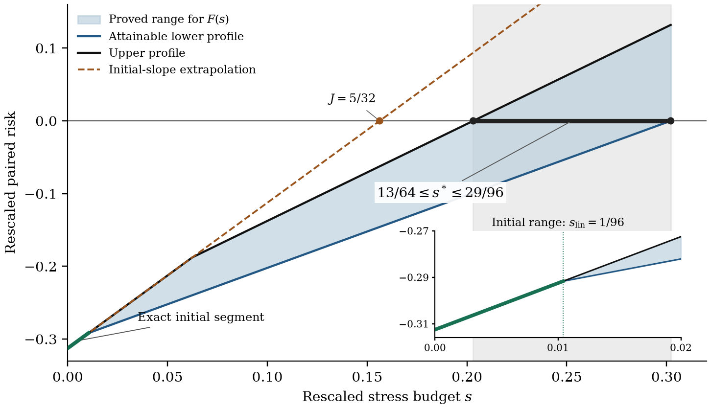
The initial linear profile holds on .
Proof. For , the negative-moment section has , so integrating over this interval gives . For , the section is empty and . Reflection gives . On the lower half of , is the smaller moment, which gives . Using then gives , and Proposition 3.2 yields . The first-coordinate kernel from (4.11) reaches zero risk at cost . For the lower bound, the midpoint potentials with give
For , the section integrations in Appendix B.2 give the first line. For , the efficiency decomposition (4.2) gives the second. Every kernel with therefore costs at least , which is above . Q.E.D.
Setting , we obtain analytical envelopes for on , where . The balanced kernel has cost , zero projected flux, and risk , and the first-coordinate comparison kernel has cost and risk zero. Their convex mixtures have affine paired risk because zero minimizes both threshold objectives for each kernel, and affine cost because the balanced kernel has zero flux. Joining these mixtures to the exact initial linear segment realizes the lower envelope
To bound from above, we invert the two threshold estimates and combine them with the efficiency bound:
The last equality holds because the branches inside the maximum meet only at . Figure 3 plots the analytical envelopes on . The guaranteed linear segment covers one fifteenth of the tangent prediction , whereas the critical coefficient lies between and times . So the initial slope is attained on a positive interval, and the required reversal budget is still at least higher than its tangent prediction.
B. A dependence family with fixed marginal laws
Section 5.1 used an independent uniform reference with background displacement twice as costly as either traded direction. We now move to the equal-effective-cost boundary to see how changing the reference dependence affects the required background share and the budget derivative . Keeping uniform marginals, , and , we perturb the independent density by the product of the centered losses and :
After rescaling the losses to , this is a one-parameter subfamily of the trivariate Farlie–Gumbel–Morgenstern family [27, Section 2]: the interactions between each traded coordinate and the background have parameter , and the other interaction parameters are zero. Centering preserves every marginal, and the parameter restriction keeps the density strictly positive on the cube. Central reflection fixes , where the section density is , so increasing reduces the section mass away from even as covariance increases. On the unchanged half-section , let , where . Set , , and denote the same-side masses by .
Proposition 5.3 (Background share along the dependence family). For , the boundary flow is attained and
In particular,
To obtain the explicit value, we use all the mass in and and match their projections in two disjoint parts of the cross-region. The section inequalities in Appendix B.3 give the required capacity throughout , and the midpoint potential gives the same value in the dual problem, so this feasible flow is optimal.
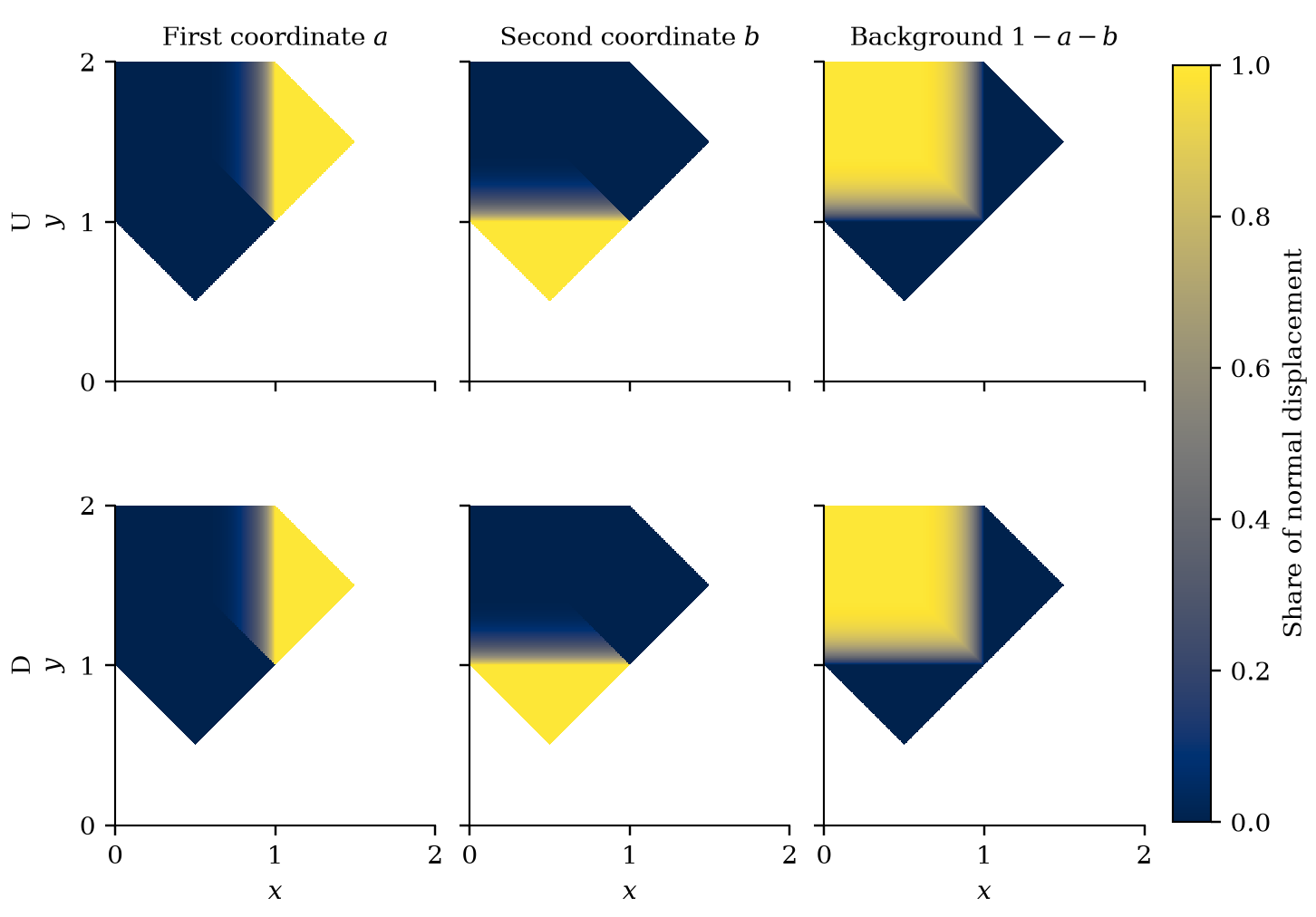
As reference dependence varies through , the minimum background share and the corresponding unnormalized displacement moment move in opposite directions:
The contrast comes from the median plane , on which the centered factors satisfy . Increasing thus favors equal signs in the full box but reduces the section density away from by the factor . Across both exchanged half-sections, the traded-coordinate matching capacity is . By (5.3), decreases faster in absolute units than this capacity, so their difference declines. In proportion, though, the matching capacity falls faster than throughout , which leaves a larger relative share for the background coordinate.
Figure 4 compares two examples: independence (, model U) and (model D). The triples are and , so the minimum background share rises from about to while its unnormalized displacement moment falls from about to .
C. Implications for reverse stress testing and further questions
Theorem 4.2 shows that an exact initial sensitivity need not predict how much dependence stress is required to reverse a diversification trade. This bears on reverse sensitivity analysis [28, 29], where the quantity of interest is the distance to a decision reversal. Under the traded-coordinate dominance condition (2.9), extrapolates an attained initial slope, yet if ,
Proposition 3.2 attains the initial slope by balancing opposite movements on selected fibers. Equality in the efficiency bound at reversal would require balancing cheapest-coordinate projections across the entire tail section, and under the stated cost condition the corner obstruction of Theorem 4.2 excludes that. Unlike optimal allocation across full Fréchet or Wasserstein ambiguity sets [23], our reverse stress test fixes a proposed trade and measures the least perturbation of a common reference law that reverses its paired ES ranking.
A whole-book comparison across reference dependence structures also has to account for the size of the nominal advantage. In the family of Section 5.2, consider the boundary perturbation . The gain-normalized critical budget and its right derivative at equal effective costs satisfy
Theorem 4.3 gives the absolute right derivative . By (5.4), increasing raises the gain-normalized response but lowers the absolute response: , so the decline in the nominal-gain scale outweighs the increase in background share. Reporting both boundary sensitivities to a risk committee separates a greater relative need for background displacement from a smaller absolute response in budget units.
Characterizing the boundaries between the active and stationary regions of an optimal kernel could help determine the full profile between the analytical envelopes, beyond the guaranteed initial linear interval. A uniform rate for , combined with the lower growth estimate in Theorem 3.3, would yield finite-trade error bounds for the critical budgets.
In the compact-box benchmark, a restoration premium can arise from dependence geometry and full marginal conservation even with bounded marginal tails. For unbounded marginals such as integrable Pareto or lognormal laws, the inverse-CDF derivative is unbounded near probability one, so the uniform displacement estimate in the recovery argument would need a tail-weighted substitute. Since one-dimensional remains the integral of the CDF discrepancy, this loss of a uniform quantile bound does not by itself imply a different restoration-cost exponent. The open problem is to control that integral jointly with the paired-risk error and determine whether the critical scale persists under suitable tail assumptions. Higher-dimensional projected-flow representations and estimation of critical budgets from loss data raise related questions, alongside recent work on ES estimation under weak tail assumptions [3].
Appendices and supporting material
This page includes the complete abstract, five main sections, all four main-text figures, and references. Technical appendices and declarations are available in the full manuscript and the GitHub repository.
References
1. P. Artzner, F. Delbaen, J.-M. Eber, and D. Heath, Coherent measures of risk, Math. Finance, 9(3) (1999), pp. 203–228, doi:10.1111/1467-9965.00068.
2. D. Bartl, S. Drapeau, J. Obłój, and J. Wiesel, Sensitivity analysis of Wasserstein distributionally robust optimization problems, Proc. R. Soc. A, 477(2256) (2021), article 20210176, doi:10.1098/rspa.2021.0176.
3. D. Bartl and S. Eckstein, Optimal nonparametric estimation of the expected shortfall risk, preprint (2026), to appear in SIAM J. Financial Math., arXiv:2405.00357v2.
4. D. Bartl and J. Wiesel, Sensitivity of multiperiod optimization problems with respect to the adapted Wasserstein distance, SIAM J. Financial Math., 14(2) (2023), pp. 704–720, doi:10.1137/22M1537746.
5. C. Bernard, X. Jiang, and R. Wang, Risk aggregation with dependence uncertainty, Insur. Math. Econ., 54 (2014), pp. 93–108, doi:10.1016/j.insmatheco.2013.11.005.
6. D. P. Bertsekas, Convex Optimization Theory, Athena Scientific, Belmont, MA, 2009, author's online edition.
7. J. Blanchet and K. Murthy, Quantifying distributional model risk via optimal transport, Math. Oper. Res., 44(2) (2019), pp. 565–600, doi:10.1287/moor.2018.0936.
8. M. Brandtner, Expected shortfall, spectral risk measures, and the aggravating effect of background risk, or: risk vulnerability and the problem of subadditivity, J. Bank. Financ., 89 (2018), pp. 138–149, doi:10.1016/j.jbankfin.2018.02.002.
9. J. Chen, E. Furman, and X. S. Lin, Static marginal expected shortfall: Systemic risk measurement under dependence uncertainty, Insur. Math. Econ., 130 (2026), article 103285, doi:10.1016/j.insmatheco.2026.103285.
10. Y. Chen, P. Liu, Y. Liu, and R. Wang, Ordering and inequalities for mixtures on risk aggregation, Math. Finance, 32(1) (2022), pp. 421–451, doi:10.1111/mafi.12323.
11. G. Dal Maso, An Introduction to -Convergence, Progress in Nonlinear Differential Equations and Their Applications 8, Birkhäuser, Boston, 1993, doi:10.1007/978-1-4612-0327-8.
12. C. De Vecchi, M. Nendel, and J. Streicher, Upper comonotonicity and risk aggregation under dependence uncertainty, Math. Finance, 36(1) (2026), pp. 118–139, doi:10.1111/mafi.70008.
13. S. Eckstein, M. Kupper, and M. Pohl, Robust risk aggregation with neural networks, Math. Finance, 30(4) (2020), pp. 1229–1272, doi:10.1111/mafi.12280.
14. S. Eckstein, G. Guo, T. Lim, and J. Obłój, Robust pricing and hedging of options on multiple assets and its numerics, SIAM J. Financial Math., 12(1) (2021), pp. 158–188, doi:10.1137/19M1286256.
15. P. Embrechts, G. Puccetti, and L. Rüschendorf, Model uncertainty and VaR aggregation, J. Bank. Financ., 37(8) (2013), pp. 2750–2764, doi:10.1016/j.jbankfin.2013.03.014.
16. P. Embrechts, B. Wang, and R. Wang, Aggregation-robustness and model uncertainty of regulatory risk measures, Finance Stoch., 19(4) (2015), pp. 763–790, doi:10.1007/s00780-015-0273-z.
17. L.-B. Fiechtner and J. Blanchet, Wasserstein distributionally robust regret optimization, preprint, 2025, revised 2026, arXiv:2504.10796v5.
18. R. Gao and A. J. Kleywegt, Data-driven robust optimization with known marginal distributions, working paper, 2017, https://faculty.mccombs.utexas.edu/rui.gao/copula.pdf.
19. R. Gao and A. J. Kleywegt, Distributionally robust stochastic optimization with Wasserstein distance, Math. Oper. Res., 48(2) (2023), pp. 603–655, doi:10.1287/moor.2022.1275.
20. J. Korman, R. J. McCann, and C. Seis, Dual potentials for capacity constrained optimal transport, Calc. Var. Partial Differential Equations, 54 (2015), pp. 573–584, doi:10.1007/s00526-014-0795-9.
21. H. Lam, Sensitivity to serial dependency of input processes: A robust approach, Manage. Sci., 64(3) (2018), pp. 1311–1327, doi:10.1287/mnsc.2016.2667.
22. L. Li, H. Shao, R. Wang, and J. Yang, Worst-case Range Value-at-Risk with partial information, SIAM J. Financial Math., 9(1) (2018), pp. 190–218, doi:10.1137/17M1126138.
23. P. Liu and Y. Liu, Portfolio diversification and concentration under dependence uncertainty: A majorization approach, preprint, 2026, arXiv:2609.04496v1.
24. R. J. Martin, Saddlepoint methods in portfolio theory, in The Oxford Handbook of Credit Derivatives, A. Lipton and A. Rennie, eds., Oxford University Press, Oxford (2011), pp. 533–569, doi:10.1093/oxfordhb/9780199546787.013.0015.
25. A. J. McNeil, R. Frey, and P. Embrechts, Quantitative Risk Management: Concepts, Techniques and Tools, revised ed., Princeton University Press, Princeton, NJ, 2015.
26. H. Namkoong, Local sensitivity under transport restrictions, preprint, 2026, arXiv:2606.04276v1.
27. S. Ota and M. Kimura, Effective estimation algorithm for parameters of multivariate Farlie–Gumbel–Morgenstern copula, Jpn. J. Stat. Data Sci., 4 (2021), pp. 1049–1078, doi:10.1007/s42081-021-00118-y.
28. S. M. Pesenti, P. Millossovich, and A. Tsanakas, Reverse sensitivity testing: What does it take to break the model?, European J. Oper. Res., 274(2) (2019), pp. 654–670, doi:10.1016/j.ejor.2018.10.003.
29. S. M. Pesenti, Reverse sensitivity analysis for risk modelling, Risks, 10(7) (2022), article 141, doi:10.3390/risks10070141.
30. S. M. Pesenti and S. Jaimungal, Portfolio optimization within a Wasserstein ball, SIAM J. Financial Math., 14(4) (2023), pp. 1175–1214, doi:10.1137/22M1496803.
31. G. Ch. Pflug and M. Pohl, A review on ambiguity in stochastic portfolio optimization, Set-Valued Var. Anal., 26(4) (2018), pp. 733–757, doi:10.1007/s11228-017-0458-z.
32. R. T. Rockafellar and S. Uryasev, Conditional value-at-risk for general loss distributions, J. Bank. Financ., 26(7) (2002), pp. 1443–1471, doi:10.1016/S0378-4266(02)00271-6.
33. L. Rüschendorf, Mathematical Risk Analysis: Dependence, Risk Bounds, Optimal Allocations and Portfolios, Springer Series in Operations Research and Financial Engineering, Springer, Berlin, Heidelberg, 2013, doi:10.1007/978-3-642-33590-7.
34. F. Santambrogio, Optimal Transport for Applied Mathematicians: Calculus of Variations, PDEs, and Modeling, Progress in Nonlinear Differential Equations and Their Applications 87, Birkhäuser, Cham, 2015, doi:10.1007/978-3-319-20828-2.
35. N. Sauldubois, Higher-order sensitivity analysis of Wasserstein and adapted Wasserstein distributionally robust optimization problems, preprint, 2026, arXiv:2609.25345v1.
36. O. Scaillet, Nonparametric estimation and sensitivity analysis of expected shortfall, Math. Finance, 14(1) (2004), pp. 115–129, doi:10.1111/j.0960-1627.2004.00184.x.
37. M. Sion, On general minimax theorems, Pacific J. Math., 8(1) (1958), pp. 171–176, doi:10.2140/pjm.1958.8.171.
38. D. Tasche, Conditional expectation as quantile derivative, preprint, 2001, arXiv:math/0104190v1.
39. S. S. Vallender, Calculation of the Wasserstein distance between probability distributions on the line, Theory Probab. Appl., 18(4) (1974), pp. 784–786, doi:10.1137/1118101.
40. C. Villani, Topics in Optimal Transportation, Graduate Studies in Mathematics 58, American Mathematical Society, Providence, RI, 2003.
41. R. Wang, V. Bignozzi, and A. Tsanakas, How superadditive can a risk measure be?, SIAM J. Financial Math., 6(1) (2015), pp. 776–803, doi:10.1137/140981046.